Download the notebook here!
Interactive online version: ![]()
Repeated observations and the estimation of causal effects
Overview
Interrupted time series models
Regression discontinuity design
Panel data
Traditional adjustment strategies
Model-based approaches
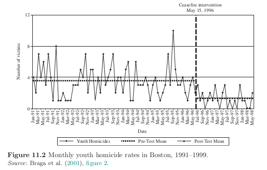
Interrupted time series models (ITS)
before the treatment is introduced (for \(t \le t^*\)), \(D_t = 0\) and \(Y_t = Y^0_t\)
after the treatment is in place (from \(t^*\) through \(T\)), \(D_t = 1\) and \(Y_t = Y^1_t\)
The causal effect of the treatment is then \(\delta_t = Y_t^1 - Y^0_t\) for time periods \(t^*\) through \(T\). This is equal to \(\delta_t = Y_t - Y^0_t\). The crucial assumption is that the obseved values of \(y_t\) before \(t^*\) can be used to speciy \(f(t)\) for all time periods, including those after treatment.
Operation Ceasefire involved meetings with gang-involved youth who were engaged in gang conflict. Gang members were offered educational, employment, and other social services if they committed to refraining from gang-related deviance.
Strategies to strengthen ITS analysis
Assess the effect of the cause on multiple outcomes that should be be affected by the cause.
Assess the effect of the cause on outcomes that should not be affected by the cause.
Assess the effect of the cause withing subgroups across which the causal effect should vary in predictable ways.
Adjust for trends in other variables that may affect or be related to the underlying time series of interest.
Assess the impact of the termination of th cause in addition to its initiation.
Panel data
We now need to add a time dimension to our effect analysis, i.e. \(Y^d_t\) for \(d = 0, 1\).
Seminal paper
Card and Krueger (1995, 2000)
We briefly discuss the exposition from Angrist & Pischke (2008).
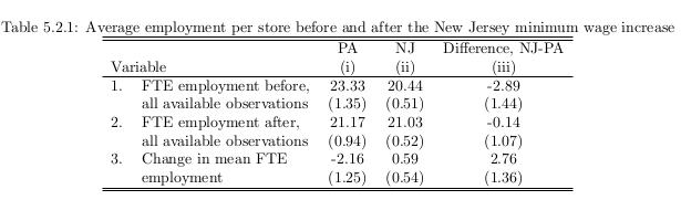
We are interested in
assuming common trend
moving to observed outcomes where T indicates period in conditioning set.
We can now map these observed objects to Table 5.2.
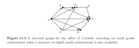
Demonstration
We consider how alterantive estimators perform assuming a world where:
no catholic elementary schools or middle schools exist
all students consider entering either public or Cathlic high schools after end of eight grade
pretretment achievement test score is available for the eights grade
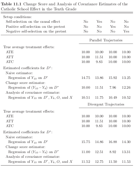
Control outcomes
There is a linear time trend for \(Y^0_{it}\) but we will also consider a diverging trend scenario.
Treated outcomes
The treatment effect increases in time.
Treatment selection
Why is the average control outcome higher among the (eventually) treated?
[8]:
num_agents, selection, trajectory = 10, "baseline", "parallel"
df = get_sample_panel_demonstration(num_agents, selection, trajectory)
df.groupby(["D_ever", "Grade"])["Y"].mean()
[8]:
D_ever  Grade
0       8              NaN
        9        97.858309
        10       98.398170
Name: Y, dtype: float64
How do our standard estimators perform in these setting?
[10]:
for selection in [
    "baseline",
    "self-selection on gains",
    "self-selection on pretest",
]:
    for trajectory in ["parallel", "divergent"]:
        print("\n Selection: {:}, Trajectory: {:}".format(selection, trajectory))
        num_agents, selection, trajectory = 1000, selection, trajectory
        df = get_sample_panel_demonstration(num_agents, selection, trajectory)
        for estimator in ["naive", "diff"]:
            rslt = get_panel_estimates(estimator, df)
            print("{:10}: {:5.3f}".format(estimator, rslt.params["D"]))
 Selection: baseline, Trajectory: parallel
naive     : 15.278
diff      : 9.416

 Selection: baseline, Trajectory: divergent
naive     : 15.363
diff      : 9.774

 Selection: self-selection on gains, Trajectory: parallel
naive     : 14.151
diff      : 11.358

 Selection: self-selection on gains, Trajectory: divergent
naive     : 15.986
diff      : 12.460

 Selection: self-selection on pretest, Trajectory: parallel
naive     : 14.082
diff      : 8.971

 Selection: self-selection on pretest, Trajectory: divergent
naive     : 16.011
diff      : 10.543
Resources
Angrist, J. D. and Pischke, J.-S. (2008). Mostly harmless econometrics: An empiricist’s companion. Princeton, NJ: Princeton University Press.
Bertrand, M., Duflo E., and Mullainathan, S. (2004). How much should we trust differences-in-differences estimates?. The Quarterly Journal of Economics, 119(1), 249-275.
Braga, A. A., Kennedy, D. M., Waring, E. J., and Piehl, A. M. (2001). Problem-oriented policing, deterrence, and youth violence: An evaluation of boston’s operation ceasefire. Journal of research in crime and delinquency, 38(3), 195–225.
Card, D., and Krueger, A. B. (1995). Time-series minimum-wage studies: A meta-analysis. The American Economic Review, 85(2), 238–243.
Card, D. and Krueger, A. B. (2000). Minimum wages and employment: A case study of the fast-food industry in new jersey and pennsylvania. American Economic Review, 90(5), 1397–1420.
Frölich, M. and Sperlich, S. (2019). Impact evaluation. Cambridge, England: Cambridge University Press.
Lechner, M. (2010). The estimation of causal effects by difference-in-difference methods, 4(3), 165–224.