Download the notebook here! Interactive online version:

Regression estimators of causal effects

Overview

• Regression as a descriptive tool

• Regression adjustment as a strategy to to estimate causal effects

• Regression as conditional-variance-weighted matching

• Regression as an implementation of a perfect stratification

• Regression as supplemental adjustment when matching

• Extensions and other perspectives

• Conclusion

We start with different ways of using regression

• descriptive tools

  • Anscombe quartet

• estimating causal effects

• Freedman’s paradox

Regression as a descriptive tool

Goldberger (1991) motivates least squares regression as a technique to estimate a best-fitting linear approximation to a conditional expectation function that may be nonlinear in the population.

Best is defined as minimizing the average squared differences between the fitted values and the true values of the conditional expectations functions.

df = get_sample_demonstration_1(num_agents=10000)
df.head()

	Y	D	S	Y_1	Y_0
0	0.113157	0	1	4.055376	0.113157
1	9.479227	0	3	14.146062	9.479227
2	0.409400	0	1	2.081023	0.409400
3	7.087262	1	2	7.087262	5.145585
4	3.338352	0	1	2.825938	3.338352

df.groupby(["D", "S"])["Y"].mean()

D  S
0  1     2.014537
   2     6.032069
   3     9.976885
1  1     4.067050
   2     8.028103
   3    14.025534
Name: Y, dtype: float64

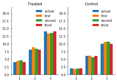
How does the functional form of the conditional expectation look like?

plot_conditional_expectation_demonstration_1(df)

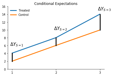
What does the difference between the two lines tell us about treatment effect heterogeneity?

We will fit four different prediction models using ordinary least squares.

\begin{align*} &\hat{Y} = \beta_0 + \beta_1 D + \beta_2 S \\ &\hat{Y} = \beta_0 + \beta_1 D + \beta_2 S_1 + \beta_3 S_2 \\ &\hat{Y} = \beta_0 + \beta_1 D + \beta_2 S_1 + \beta_3 S_2 + \beta_4 S_1 * D + \beta_5 S_2 * D \end{align*}

rslt = smf.ols(formula="Y ~ D + S", data=df).fit()
rslt.summary()

OLS Regression Results

Dep. Variable:	Y	R-squared:	0.941
Model:	OLS	Adj. R-squared:	0.941
Method:	Least Squares	F-statistic:	8.018e+04
Date:	Tue, 26 May 2020	Prob (F-statistic):	0.00
Time:	07:30:39	Log-Likelihood:	-15339.
No. Observations:	10000	AIC:	3.068e+04
Df Residuals:	9997	BIC:	3.071e+04
Df Model:	2
Covariance Type:	nonrobust

	coef	std err	t	P>|t|	[0.025	0.975]
Intercept	-2.6594	0.027	-98.877	0.000	-2.712	-2.607
D	2.7202	0.025	108.756	0.000	2.671	2.769
S	4.4181	0.014	311.459	0.000	4.390	4.446

Omnibus:	1.627	Durbin-Watson:	2.023
Prob(Omnibus):	0.443	Jarque-Bera (JB):	1.637
Skew:	0.016	Prob(JB):	0.441
Kurtosis:	2.946	Cond. No.	6.15

Warnings:
[1] Standard Errors assume that the covariance matrix of the errors is correctly specified.

df["predict"] = rslt.predict()
df.groupby(["D", "S"])[["Y", "predict"]].mean()

		Y	predict
D	S
0	1	2.014537	1.758657
	2	6.032069	6.176733
	3	9.976885	10.594808
1	1	4.067050	4.478865
	2	8.028103	8.896941
	3	14.025534	13.315017

plot_predictions_demonstration_1(df)

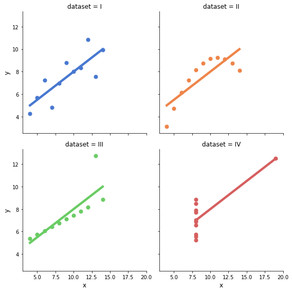
Anscombe quartet

The best linear approximation can be the same for very different functions. The Anscombe quartet (Anscombe, 1973) and many other useful datasets are available in statsmodels as part of the Datasets Package.

df1, df2, df3, df4 = get_anscombe_datasets()
for i, df in enumerate([df1, df2, df3, df4]):
    rslt = smf.ols(formula="y ~ x", data=df).fit()
    print(f"\n Dataset {i}")
    print(" Intercept: {:5.3f} x: {:5.3f}".format(*rslt.params))

 Dataset 0
 Intercept: 3.000 x: 0.500

 Dataset 1
 Intercept: 3.001 x: 0.500

 Dataset 2
 Intercept: 3.002 x: 0.500

 Dataset 3
 Intercept: 3.002 x: 0.500

So what does the data behind these regressions look like?

plot_anscombe_dataset()

Regression adjustment as a strategy to estimate causal effects

Regression models and omitted-variable bias

\begin{align*} Y = \alpha + \delta D + \epsilon \end{align*}

• \(\delta\) is interpreted as an invariant, structural causal effect that applies to all members of the population.

• \(\epsilon\) is a summary random variable that represents all other causes of \(Y\).

\begin{align*} \hat{\delta}_{OLS, \text{bivariate}} = \frac{Cov_N(y_i, d_i)}{Var_N(d_i)} \end{align*}

It now depends on the correlation between \(\epsilon\) and \(D\) whether \(\hat{\delta}\) provides an unbiased and consistent estimate of the true causal effect

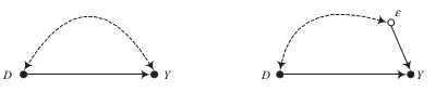
We now move to the potential outcomes model to clarify the connection between omitted-variable bias and self-selection bias.

Potential outcomes and omitted-variable bias

\begin{align*} Y = \underbrace{\mu^0}_{\alpha} + \underbrace{(\mu^1 - \mu^0)}_{\delta} D + \underbrace{\{\nu^0 + D(\nu^1 - \nu^0 )\}}_{\epsilon}, \end{align*}

where \(\mu^0\equiv E[Y^0]\), \(\mu^1\equiv E[Y^1]\), \(\nu^0\equiv Y^0 - E[Y^0]\), and \(\nu^1\equiv Y^1 - E[Y^1]\).

What induces a correlation between \(D\) an \(\{\nu^0 + D(\nu^1 - \nu^0 )\}\)?

• baseline bias, there is a net baseline difference in the hypothetical no-treatment state that is correlated with treatment uptake \(\rightarrow\) \(D\) is correlated with \(\nu_0\)

• differential treatment bias, there is a net treatment effect difference that is correlated with treatment uptake \(\rightarrow\) \(D\) is correlated with \(D(\nu^1 - \nu^0 )\)

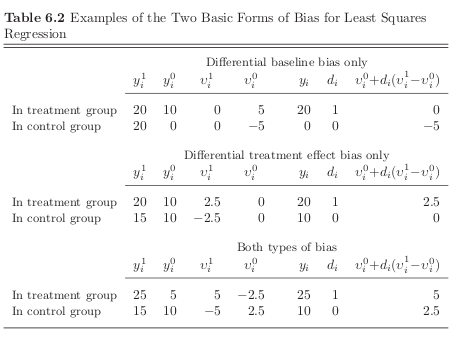
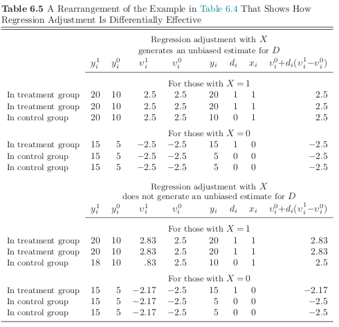
Errata

Please note that there is a relevant correction on the author’s website:

• page 198, Table 6.2, first panel: In order to restrict the bias to differential baseline bias only, as required by the label on the first panel of the table, replace 20 with 10 in the first cell of the second row.Then, carry the changes across columns so that (a) the values for \(\nu^1_i\) are 5 for the individual in the treatment group and -5 for the individual in the control group and (b) the value for \({\nu^0_i + D(\nu^1_i − \nu^0_i)}\) is 5 for the individual in the treatment group

Group	\(y_i^1\)	\(y_i^0\)	\(\nu_i^1\)	\(\nu_i^0\)	\(y_i\)	\(d_i\)	\(\nu_i^1 + d_i (\nu_i^1 - \nu_i^0)\)	$ d_i (\nu_i^1 - \nu_i^0)$
Treated	20	10	5	5	20	1	5.000000000000000000000000	0.000000000
Control	10	0	-5	-5	0	0	-5	0.000000000

Regression as adjustment for otherwise omitted variables

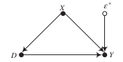
We first want to illustrate how we can subtract out the dependence between \(D\) and \(Y\) induced by their common determinant \(X\). Let’s quickly simulate a parameterized example:

\begin{align*} D & = I[X + \eta > 0] \\ Y & = D + X + \epsilon, \end{align*}

where \((\eta, \epsilon)\) follow a standard normal distribution.

df = get_quick_sample(num_samples=1000)

We now first run a complete regression.

stat = smf.ols(formula="Y ~ D + X", data=df).fit().params[1]
print(f"Estimated effect: {stat:5.3f}")

Estimated effect: 0.924

However, as it turns out, we can also get the identical estimate by first partialling out the effect of \(X\) on \(D\) as well as \(Y\).

df_resid = pd.DataFrame(columns=["Y_resid", "D_resid"])
for label in ["Y", "D"]:
    column, formula = f"{label}_resid", f"{label} ~ X"
    df_resid.loc[:, column] = smf.ols(formula=formula, data=df).fit().resid

smf.ols(formula="Y_resid ~ D_resid", data=df_resid).fit().params[1]
print(f"Estimated effect: {stat:5.3f}")

Estimated effect: 0.924

We will now look at two datasets that are observationally equivalent but regression adjustment for observable \(X\) does only work in one of them.

Note

• The naive estimates will be identical as the observed values \(y_i\) and \(d_i\) are the same.

for sample in range(2):

    df = get_sample_regression_adjustment(sample)
    print("Sample {:}\n".format(sample))

    stat = (df["Y_1"] - df["Y_0"]).mean()
    print("True effect:    {:5.4f}".format(stat))

    stat = df.query("D == 1")["Y"].mean() - df.query("D == 0")["Y"].mean()
    print("Naive estimate: {:5.4f}".format(stat))

    rslt = smf.ols(formula="Y ~ D", data=df).fit()
    print(rslt.summary())

Sample 0

True effect:    10.0000
Naive estimate: 11.6540
                            OLS Regression Results
==============================================================================
Dep. Variable:                      Y   R-squared:                       0.860
Model:                            OLS   Adj. R-squared:                  0.860
Method:                 Least Squares   F-statistic:                     6113.
Date:                Tue, 26 May 2020   Prob (F-statistic):               0.00
Time:                        11:44:40   Log-Likelihood:                -2275.1
No. Observations:                1000   AIC:                             4554.
Df Residuals:                     998   BIC:                             4564.
Df Model:                           1
Covariance Type:            nonrobust
==============================================================================
                 coef    std err          t      P>|t|      [0.025      0.975]
------------------------------------------------------------------------------
Intercept      6.8379      0.105     65.272      0.000       6.632       7.044
D             11.6540      0.149     78.187      0.000      11.361      11.946
==============================================================================
Omnibus:                     7278.240   Durbin-Watson:                   1.966
Prob(Omnibus):                  0.000   Jarque-Bera (JB):               94.873
Skew:                          -0.097   Prob(JB):                     2.50e-21
Kurtosis:                       1.504   Cond. No.                         2.60
==============================================================================

Warnings:
[1] Standard Errors assume that the covariance matrix of the errors is correctly specified.
Sample 1

True effect:    9.6280
Naive estimate: 11.6540
                            OLS Regression Results
==============================================================================
Dep. Variable:                      Y   R-squared:                       0.860
Model:                            OLS   Adj. R-squared:                  0.860
Method:                 Least Squares   F-statistic:                     6113.
Date:                Tue, 26 May 2020   Prob (F-statistic):               0.00
Time:                        11:44:42   Log-Likelihood:                -2275.1
No. Observations:                1000   AIC:                             4554.
Df Residuals:                     998   BIC:                             4564.
Df Model:                           1
Covariance Type:            nonrobust
==============================================================================
                 coef    std err          t      P>|t|      [0.025      0.975]
------------------------------------------------------------------------------
Intercept      6.8379      0.105     65.272      0.000       6.632       7.044
D             11.6540      0.149     78.187      0.000      11.361      11.946
==============================================================================
Omnibus:                     7278.240   Durbin-Watson:                   1.966
Prob(Omnibus):                  0.000   Jarque-Bera (JB):               94.873
Skew:                          -0.097   Prob(JB):                     2.50e-21
Kurtosis:                       1.504   Cond. No.                         2.60
==============================================================================

Warnings:
[1] Standard Errors assume that the covariance matrix of the errors is correctly specified.

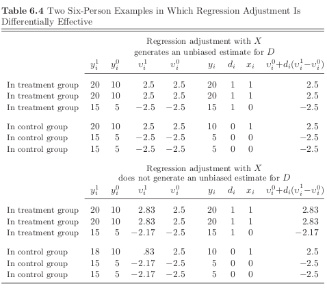
Now we condition on \(X\) to see where conditioning might help in obtaining an unbiased estimate of the true effect. Note that the treatment effect \((y^1_i - y^0_i)\) is uncorrelated with \(d_i\) within each strata of \(X\) in the first example. That is not true in the second example.

for sample in range(2):

    df = get_sample_regression_adjustment(sample)
    print("Sample {:}\n".format(sample))

    stat = (df["Y_1"] - df["Y_0"]).mean()
    print(f"True effect:{stat:24.4f}")

    stat = df.query("D == 1")["Y"].mean() - df.query("D == 0")["Y"].mean()
    print(f"Naive estimate:{stat:21.4f}")

    rslt = smf.ols(formula="Y ~ D + X", data=df).fit()
    print(f"Conditional estimate:{rslt.params[1]:15.4f}\n")

Sample 0

True effect:                 10.0000
Naive estimate:              11.6540
Conditional estimate:        10.0000

Sample 1

True effect:                  9.6280
Naive estimate:              11.6540
Conditional estimate:        10.0000

To summarize: Regression adjustment by \(X\) will yield a consistent and unbiased estimate of the ATE when:

• \(D\) is mean independent of (and therefore uncorrelated with) \(v^0 + D(v^1 - v^0)\) for each subset of respondent identified by distinct values on the variables in \(X\)

• the causal effect of \(D\) does not vary with \(X\)

• a fully flexible parameterization of \(X\) is used

Freedman’s paradox

Let’s explore some of the challenges of finding the right regression specification.

In statistical analysis, Freedman’s paradox (Freedman, 1983), named after David Freedman, is a problem in model selection whereby predictor variables with no relationship to the dependent variable can pass tests of significance – both individually via a t-test, and jointly via an F-test for the significance of the regression. (Wikipedia)

We fill a dataframe with random numbers. Thus there is no causal relationship between the dependent and independent variables.

columns = ["Y"]
[columns.append("X{:}".format(i)) for i in range(50)]
df = pd.DataFrame(np.random.normal(size=(100, 51)), columns=columns)

Now we run a simple regression of the random independent variables on the dependent variable.

formula = "Y ~ " + " + ".join(columns[1:])
rslt = smf.ols(formula=formula, data=df).fit()
rslt.summary()

OLS Regression Results

Dep. Variable:	Y	R-squared:	0.545
Model:	OLS	Adj. R-squared:	0.081
Method:	Least Squares	F-statistic:	1.176
Date:	Tue, 26 May 2020	Prob (F-statistic):	0.286
Time:	11:32:24	Log-Likelihood:	-108.43
No. Observations:	100	AIC:	318.9
Df Residuals:	49	BIC:	451.7
Df Model:	50
Covariance Type:	nonrobust

	coef	std err	t	P>|t|	[0.025	0.975]
Intercept	0.1106	0.136	0.811	0.421	-0.163	0.384
X0	-0.0922	0.222	-0.416	0.679	-0.538	0.353
X1	-0.1713	0.141	-1.217	0.229	-0.454	0.111
X2	-0.0741	0.155	-0.478	0.635	-0.386	0.237
X3	0.1575	0.134	1.178	0.244	-0.111	0.426
X4	0.2736	0.172	1.595	0.117	-0.071	0.618
X5	-0.0649	0.172	-0.378	0.707	-0.410	0.280
X6	0.0063	0.141	0.045	0.964	-0.276	0.289
X7	0.1089	0.141	0.774	0.443	-0.174	0.392
X8	0.0694	0.139	0.500	0.619	-0.210	0.348
X9	0.3075	0.149	2.059	0.045	0.007	0.608
X10	0.0189	0.168	0.113	0.911	-0.318	0.356
X11	-0.2898	0.178	-1.626	0.110	-0.648	0.068
X12	0.0207	0.129	0.160	0.873	-0.239	0.280
X13	0.0901	0.119	0.757	0.453	-0.149	0.329
X14	-0.1296	0.154	-0.843	0.403	-0.439	0.179
X15	0.0618	0.153	0.405	0.687	-0.245	0.368
X16	-0.1151	0.122	-0.944	0.350	-0.360	0.130
X17	0.1265	0.170	0.744	0.460	-0.215	0.468
X18	0.1578	0.140	1.129	0.264	-0.123	0.439
X19	-0.0752	0.157	-0.477	0.635	-0.392	0.241
X20	-0.1454	0.133	-1.097	0.278	-0.412	0.121
X21	0.1507	0.150	1.005	0.320	-0.151	0.452
X22	0.4160	0.133	3.123	0.003	0.148	0.684
X23	-0.1169	0.156	-0.750	0.457	-0.430	0.196
X24	-0.2271	0.165	-1.376	0.175	-0.559	0.104
X25	0.1651	0.172	0.962	0.341	-0.180	0.510
X26	0.1461	0.123	1.192	0.239	-0.100	0.392
X27	-0.2343	0.139	-1.685	0.098	-0.514	0.045
X28	0.0508	0.138	0.368	0.715	-0.227	0.329
X29	-0.0187	0.191	-0.098	0.922	-0.403	0.365
X30	0.2245	0.149	1.511	0.137	-0.074	0.523
X31	0.0353	0.146	0.242	0.810	-0.258	0.329
X32	0.0666	0.152	0.438	0.663	-0.239	0.372
X33	-0.0281	0.151	-0.186	0.853	-0.331	0.275
X34	0.0204	0.141	0.144	0.886	-0.263	0.304
X35	-0.1940	0.138	-1.409	0.165	-0.471	0.083
X36	0.1215	0.144	0.843	0.403	-0.168	0.411
X37	0.3450	0.171	2.023	0.049	0.002	0.688
X38	0.2652	0.148	1.787	0.080	-0.033	0.563
X39	0.0370	0.167	0.221	0.826	-0.299	0.373
X40	-0.0072	0.147	-0.049	0.961	-0.302	0.288
X41	0.2258	0.154	1.469	0.148	-0.083	0.535
X42	-0.1910	0.154	-1.242	0.220	-0.500	0.118
X43	0.1973	0.139	1.423	0.161	-0.081	0.476
X44	-0.1017	0.136	-0.750	0.457	-0.374	0.171
X45	-0.1656	0.137	-1.210	0.232	-0.441	0.109
X46	-0.0255	0.152	-0.168	0.867	-0.330	0.279
X47	0.1621	0.148	1.094	0.279	-0.136	0.460
X48	0.1768	0.144	1.228	0.225	-0.113	0.466
X49	0.1961	0.146	1.345	0.185	-0.097	0.489

Omnibus:	0.122	Durbin-Watson:	2.167
Prob(Omnibus):	0.941	Jarque-Bera (JB):	0.302
Skew:	-0.007	Prob(JB):	0.860
Kurtosis:	2.731	Cond. No.	6.59

Warnings:
[1] Standard Errors assume that the covariance matrix of the errors is correctly specified.

We use this to inform a second regression where we only keep the variables that were significant at the 25% level.

final_covariates = list()
for label in rslt.params.keys():
    if rslt.pvalues[label] > 0.25:
        continue
    final_covariates.append(label)

formula = "Y ~ " + " + ".join(final_covariates)
rslt = smf.ols(formula=formula, data=df).fit()
rslt.summary()

OLS Regression Results

Dep. Variable:	Y	R-squared:	0.402
Model:	OLS	Adj. R-squared:	0.260
Method:	Least Squares	F-statistic:	2.834
Date:	Tue, 26 May 2020	Prob (F-statistic):	0.000627
Time:	07:19:03	Log-Likelihood:	-122.11
No. Observations:	100	AIC:	284.2
Df Residuals:	80	BIC:	336.3
Df Model:	19
Covariance Type:	nonrobust

	coef	std err	t	P>|t|	[0.025	0.975]
Intercept	0.0853	0.103	0.832	0.408	-0.119	0.289
X1	-0.0874	0.099	-0.879	0.382	-0.285	0.111
X3	0.1712	0.101	1.698	0.093	-0.029	0.372
X4	0.1905	0.111	1.710	0.091	-0.031	0.412
X9	0.2888	0.104	2.768	0.007	0.081	0.496
X11	-0.2161	0.119	-1.812	0.074	-0.453	0.021
X22	0.3742	0.100	3.735	0.000	0.175	0.574
X24	-0.2796	0.103	-2.716	0.008	-0.484	-0.075
X26	0.1391	0.094	1.484	0.142	-0.047	0.326
X27	-0.2348	0.103	-2.283	0.025	-0.439	-0.030
X30	0.1220	0.110	1.109	0.271	-0.097	0.341
X35	-0.1628	0.093	-1.742	0.085	-0.349	0.023
X37	0.2214	0.100	2.206	0.030	0.022	0.421
X38	0.2400	0.106	2.267	0.026	0.029	0.451
X41	0.0482	0.102	0.471	0.639	-0.155	0.252
X42	-0.1669	0.113	-1.478	0.143	-0.392	0.058
X43	0.1723	0.096	1.786	0.078	-0.020	0.364
X45	-0.1853	0.101	-1.838	0.070	-0.386	0.015
X48	0.1667	0.092	1.811	0.074	-0.016	0.350
X49	0.1491	0.100	1.492	0.140	-0.050	0.348

Omnibus:	2.282	Durbin-Watson:	2.259
Prob(Omnibus):	0.319	Jarque-Bera (JB):	1.718
Skew:	0.137	Prob(JB):	0.424
Kurtosis:	2.420	Cond. No.	2.43

Warnings:
[1] Standard Errors assume that the covariance matrix of the errors is correctly specified.

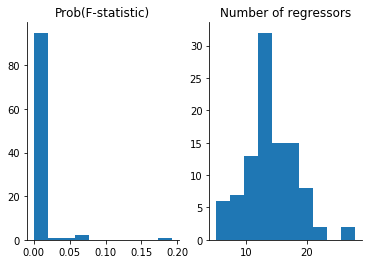
What to make of this exercise?

np.random.seed(213)

df = pd.DataFrame(columns=["F-statistic", "Regressors"])
for i in range(100):
    model = run_freedman_exercise()
    df["Regressors"].loc[i] = len(model.params)
    df["F-statistic"].loc[i] = model.f_pvalue

plot_freedman_exercise(df)

Resources

• Goldberger, A. S. (1991). A course in econometrics. Cambridge, MA: Harvard University Press.

• F. J. Anscombe (1973). Graphs in Statistical Analysis. The American Statistician, 27, 17–21.

• Freedman, David A.; Freedman, David A. (1983). A Note on Screening Regression Equations. The American Statistician. 37 (2), 152–155.