Download the notebook here!
Interactive online version: ![]()
Potential outcome model
Introduction
Given what we know from the introduction about the potential outcome model, we will initially prepare the Lalonde Dataset to fit the framework and use it as a running example going forward.
What are this example’s …
potential outcomes
counterfactual state
treatment
[2]:
df = get_lalonde_data()
df.head()
[2]:
| treat | re78 | Y | Y_0 | Y_1 | D | |
|---|---|---|---|---|---|---|
| 101 | 1 | 9970.681 | 9970.681 | NaN | 9970.681 | 1 |
| 611 | 0 | 7094.920 | 7094.920 | 7094.920 | NaN | 0 |
| 396 | 0 | 11223.720 | 11223.720 | 11223.720 | NaN | 0 |
| 681 | 0 | 4687.937 | 4687.937 | 4687.937 | NaN | 0 |
| 397 | 0 | 5088.760 | 5088.760 | 5088.760 | NaN | 0 |
We are dealing with a binary treatment here: \(D = 1\) if the individual did participate in the training program and \(D = 0\) if it did not. However, in practice assigning treatment is never that easy. We lump a lot of heterogeneity together (e.g. different sites, content of curriculum) that might affect the success of program participation. Maybe we should stratify the analysis by site?
Individual-specific effect of treatment
It would be great if we could get our hands on the individual-specific effect of treatment.
Why do individuals have potentially different effects of treatment?
[3]:
fig, ax = plt.subplots()
x = np.linspace(-5, 5, 5000)
pdf = ss.norm.pdf(x, 0, 1)
ax.plot(x, pdf)
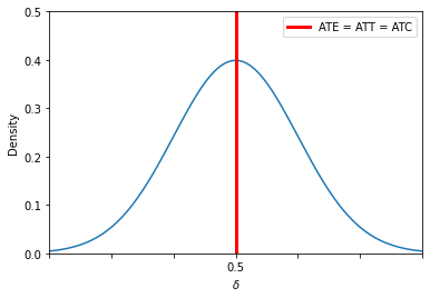
ax.set_xlabel(r"$\delta = Y^1 - Y^0$")
ax.set_ylabel("Density")
x_formatter = FixedFormatter(["", "", "", 0.5, "", "", ""])
x_locator = FixedLocator([-3, -2, -1, 0, 1, 2, 3])
ax.xaxis.set_major_locator(x_locator)
ax.xaxis.set_major_formatter(x_formatter)
ax.set_xlim([-3, 3])
ax.set_ylim([0, 0.5])
[3]:
(0.0, 0.5)
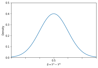
There might be considerable heterogeneity in the benefits of treatment among the population. And summarizing the distribution of benefits with a single number, for example \(E[\delta]\), might result in a loss of information.
Examples
medical treatment
Give our definitions of \((Y^1, Y^0, D)\) and their individual realizations \((y^1_i, y^0_i, d_i)\) we can now define the observed outcome \(Y\) in terms of them.
or more compactly in switching-regime notation
This leads Holland (1986) to describe the fundamental problem of causal inference:
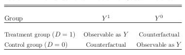
\(\rightarrow\) as only the diagonal of the table is observable we cannot simply compute \(\delta_i\) by taking the difference in potential outcomes \((y^1_i, y^0_i)\).
[4]:
df.head()
[4]:
| treat | re78 | Y | Y_0 | Y_1 | D | |
|---|---|---|---|---|---|---|
| 101 | 1 | 9970.681 | 9970.681 | NaN | 9970.681 | 1 |
| 611 | 0 | 7094.920 | 7094.920 | 7094.920 | NaN | 0 |
| 396 | 0 | 11223.720 | 11223.720 | 11223.720 | NaN | 0 |
| 681 | 0 | 4687.937 | 4687.937 | 4687.937 | NaN | 0 |
| 397 | 0 | 5088.760 | 5088.760 | 5088.760 | NaN | 0 |
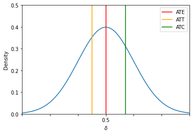
Population-level parameters
It looks like we need to give up any hope of obtaining the individual-specific effect of treatment. But what can we still hope for?
\(\rightarrow\) population-level parameters
What are common examples?
What are the policy questions they address?
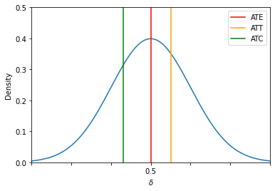
What is their relationship to each other?
[5]:
plot_individual_specific_effects(with_parameters=[0, 0.7, -0.5])
[6]:
plot_individual_specific_effects(with_parameters=[0, -0.7, 0.5])
[6]:
plot_individual_specific_effects(with_parameters=[0, 0, 0])
Stable unit treatment value assumption
The potential outcome model gets its empirical tractability when combined with the Stable Unit Treatment Value Assumption (SUTVA) of which there exist many formulations. We will go with the one from Imbens and Rubin (2015):
The potential outcomes for any unit do not vary with the treatments assigned to other units, and, for each unit there are no different forms or versions of each treatment level, which lead to different potential outcomes.
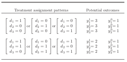
The table below shows all possible assignment patterns for a hypothetical treatment where the only constraint is that at least one individual remains in the treatment and control group. As we increase participation from one to two individuals, the potential outcome \(Y_1\) declines.
When do we need to expect this is violated?
influence patterns that result from contact across individuals in social or physical space
dilution / concentration patterns that one can assume would result from changes in the prevalence of treatment
Treatment assignment and observational studies
randomized experiment
observational study
A observational study is an empirical investigation of treatments, policies, or exposures and the effects they cause, but it differs from an experiment in that the investigator cannot control the assignment of treatments to subjects. (Rosenbaum (2002))
Naive estimation of average causal effects
We will now first outline the problem with the naive estimation of average causal effects. Then we take a closer look at the different sources of biases involved and finally discuss the set of assumptions used to *solve* these issues.
We can further decompose the average treatment effect by treatment status as the individual assignment is mutually exclusive.
The average treatment effect is a function of five unknowns. Which components can be easily computed from data?
Biases
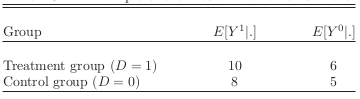
The additional information provided in the text states that \(\pi = 0.3\) meaning that 30% of the sample participate in the treatment.
Now we are ready to calculate the average treatment effect:
Next, we can determine the different components of the bias.
There are several different representation of the bias when using the naive estimator of mean difference in observed outcomes by treatment status as an estimate for the effect of treatment. We continue with the exposition in Frölich & Sperlich (2019) and Heckman, Urzua, & Vytlacil (2006).
Now we can simply add and subtract \(E[Y_1 - Y_0]\) to get the more economic version.
Sorting on levels is simply a different phrase for selection bias.
The exposition in our core textbook is slightly different. Here the term bias has two separate components which are baseline bias and differential treatment effect bias. See the discussion in the book in the subsection on the typical inconsistency and bias of the naive estimator. The term baseline bias refers to the concept of sorting and levels and selection bias.
Differential treatment bias is defined as:
The last term is derived derived from the term describing selection on gains by the following decomposition.
It is interpreted as the difference in effects between treated and control weighted by the share of control individuals. It is probably best thought of as an increment to the first term describing the average effect of treatment.
Assumptions
So, the SUTVA assumption is only necessary but not sufficient to learn about the effect of treatment in light of the biases discussed above. We are still stuck with several unknowns that we need to compute the average effect of treatment.
Consider the following two assumptions:
and recall our naive estimate
What assumptions suffice to estimate the ATE with the naive estimator?
about potential outcomes for subsets of the population
about the treatment selection / assignment process
Missing data and imputation
This is an adopted example from Imbens & Rubin (2015).
[84]:
df = get_lalonde_data()
df.head()
[84]:
| treat | re78 | Y | Y_0 | Y_1 | D | |
|---|---|---|---|---|---|---|
| 100 | 1 | 0.000 | 0.000 | NaN | 0.0 | 1 |
| 561 | 0 | 5670.820 | 5670.820 | 5670.820 | NaN | 0 |
| 130 | 1 | 0.000 | 0.000 | NaN | 0.0 | 1 |
| 318 | 0 | 0.000 | 0.000 | 0.000 | NaN | 0 |
| 687 | 0 | 7659.218 | 7659.218 | 7659.218 | NaN | 0 |
We can impute the missing values simply by their average counterpart.
[71]:
is_treated = df["D"] == 1

df.loc[~is_treated, "Y_1"] = df.loc[is_treated, "Y"].mean()
df.loc[is_treated, "Y_0"] = df.loc[~is_treated, "Y"].mean()
[50]:
df.head()
[50]:
| treat | re78 | Y | Y_0 | Y_1 | D | |
|---|---|---|---|---|---|---|
| 479 | 0 | 6930.336 | 6930.336 | 6930.336 | NaN | 0 |
| 480 | 0 | 3795.799 | 3795.799 | 3795.799 | NaN | 0 |
| 343 | 0 | 0.000 | 0.000 | 0.000 | NaN | 0 |
| 690 | 0 | 2652.625 | 2652.625 | 2652.625 | NaN | 0 |
| 70 | 1 | 0.000 | 0.000 | NaN | 0.0 | 1 |
[72]:
initial_stat = (df["Y_1"] - df["Y_0"]).mean()
print(f"Our estimated treatment effect is {initial_stat:10.2f}")
Our estimated treatment effect is 886.30
However, this does not really account for any uncertainty in our estimate. Can we do better? We now switch to the imputation of the counterfactual outcome on the individual level.
[80]:
np.random.seed(123)  # set seed to ensure reproducibility
df = get_lalonde_data()  # get the original data

status_counts = df["D"].value_counts().to_dict()

stats = list()
for _ in range(100):
    y_1_sampled = df["Y_1"].dropna().sample(n=status_counts[0], replace=True).values
    y_0_sampled = df["Y_0"].dropna().sample(n=status_counts[1], replace=True).values

    df_boot = df.copy()

    is_treated = df_boot["D"] == 1
    df_boot.loc[is_treated, "Y_0"] = y_0_sampled
    df_boot.loc[~is_treated, "Y_1"] = y_1_sampled

    stat = (df_boot["Y_1"] - df_boot["Y_0"]).mean()
    stats.append(stat)
print(f"Our estimated treatment effect is {np.mean(stats):10.2f}")
Our estimated treatment effect is 907.86
How does the full distribution of estimates look like?
[74]:
fig, ax = plt.subplots()
ax.hist(stats)
ax.set_xlabel("Statistic")
ax.set_ylabel("Frequency")
ax.vlines(initial_stat, 0, 30, linestyles="--", label="Initial", color="lightgrey")
ax.legend()
[74]:
<matplotlib.legend.Legend at 0x1e0ed15f7c0>
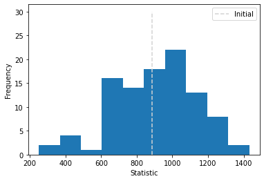
Still some limitations remains. For example, we do sample from the empirical distribution of the observed outcomes and not the actual distribution. Phrased differently, we treat the distribution of potential outcomes as known and abstract from any uncertainty in our knowledge about it.
Extensions of the binary potential outcome model
over-time potential outcomes and causal effects
a single unit over time (time series data)
many units over time (panel data)
many-valued treatments
Over-time potential outcomes
We explore the case of a single unit over time.
Ingredients
discrete time periods, \(t\in\{1, ..., T\}\)
sequence of observed values, \(\{y_1, y_2, ..., y_T\}\)
treatment initiated in \(t^*\)
duration of treatment \(k\)
Setting up the potential outcome model to explore the basic features of before-and-after designs for a single unit of analsysis.
before the treatment is introduced (for \(t < t^*\)):
while the treatment is in place (from \(t^*\) through \(t^* + k\)):
after the treatment ends (for time periods \(t > (t^* + k)\)):
\begin{align*} D_t & = 0 \\ Y_t & = Y^0_t\\ Y^1_t & \text{exists but is counterfactual} \end{align*}
The following is an adapted example from our textbook.
Year of the fire horse
We study the effect of Japanese folk belief that families who give birth to babies will suffer untold miseries. This example does not only illustrative the versatility of the potential outcome framework but also serves as an example that different approaches (informed by domain-expertise) can result in different reasonable imputations for the counterfactual outcome.
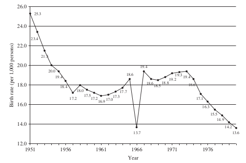
The treatment indicator is as follows: \(D_{1966} = 1\) and \(D_{\neq 1966} = 0\) and we are interested in its effect on the birth rate in Japan
A reasonable approach is to estimate it by:
[85]:
df = pd.read_csv("material/world_bank.csv", skiprows=4)
df.set_index("Country Code", inplace=True)
df.drop(["Indicator Name", "Indicator Code"], axis=1, inplace=True)

df = df.loc["JPN", "1960":"2017"]
df = df.to_frame()
df.index.name = "Year"
df.columns = ["Birth rate"]

df.sort_index(inplace=True)
df.index = df.index.astype(int)
df.head()
[85]:
| Birth rate | |
|---|---|
| Year | |
| 1960 | 17.3 |
| 1961 | 17 |
| 1962 | 17.1 |
| 1963 | 17.4 |
| 1964 | 17.8 |
Let’s get to work.
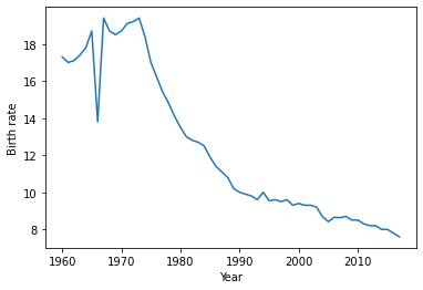
[86]:
fig, ax = plt.subplots()
ax.plot(df["Birth rate"].index, df["Birth rate"])
ax.set_ylabel("Birth rate")
ax.set_xlabel("Year")
[86]:
Text(0.5, 0, 'Year')
[87]:
df.loc[slice(1960, 1970), "Birth rate"]
[87]:
Year
1960    17.3
1961      17
1962    17.1
1963    17.4
1964    17.8
1965    18.7
1966    13.8
1967    19.4
1968    18.7
1969    18.5
1970    18.7
Name: Birth rate, dtype: object
We can just take the year before or after treatment?
[88]:
estimates = list()
for label, year in [("before", 1965), ("after", 1967)]:
    y_0 = df.loc[year, "Birth rate"]
    y_1 = df.loc[1966, "Birth rate"]
    print(f" Using the year {label}, the treatment effect is {y_1 - y_0:10.5f}")
    estimates.append(y_1 - y_0)
 Using the year before, the treatment effect is   -4.90000
 Using the year after, the treatment effect is   -5.60000
Among demographers, there is the consensus that taking the average of 1963 and 1969 the way to go instead.
[89]:
y_0 = df.loc[[1963, 1969], "Birth rate"].mean()
y_1 = df.loc[1966, "Birth rate"]
print(" Another treatment effect is {:10.5f}".format(y_1 - y_0))
estimates.append(y_1 - y_0)
Another treatment effect is -4.15000
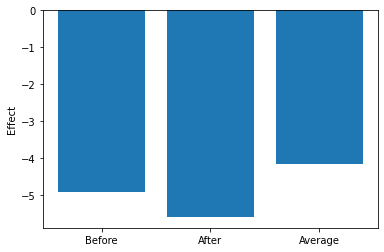
Now we have multiple effects of treatment. Which is it?
[90]:
labels = ["Before", "After", "Average"]
fig, ax = plt.subplots()
ax.bar(labels, estimates)
ax.set_ylabel("Effect")
[90]:
Text(0, 0.5, 'Effect')
Additional resources
Imbens, G. W. (2020). Potential outcome and directed acyclic graph approaches to causality: Relevance for empirical practice in economics, Journal of Economic Literature, 58(4), 1129-79.
Resources
Frölich, M., and Sperlich, S. (2019) . Impact evaluation: Treatment effects and causal analysis. Cambridge, England: Cambridge University Press.
Heckman, J. J., Urzua, S. and Vytlacil, E. (2006). Understanding instrumental variables in models with essential heterogeneity. Review of Economics and Statistics, 88(3), 389–432.
Holland, P. W. (1986). Statistics and causal inference. Journal of the American Statistical Association, 81(396), 945–960.
Imbens, G. W., and Rubin, D. B. (2015). Causal inference in statistics, social, and biomedical sciences. New York, NY: Cambridge University Press.
Rosenbaum, P. R. (2002). Overt bias in observational studies. Observational studies, 71–104.